This post assumes basic familiarity with Turing machines, P, NP, NP-completeness, decidability, and undecidability. Don’t hesitate to contact me via email if you need further clarification. Without further ado, let’s dive in.
Introduction
Why do we need reductions?
From Archimedes terrorizing the good folk of ancient Syracuse to Newton watching apples fall during a medieval plague, science has always progressed one ‘Eureka!’ at a time. Romantic as these anecdotes may be, for mathematics, we can hardly look to Mother Nature for providing us the key insight to our proofs.
Therefore, we must develop principled approaches and techniques to solve new and unseen problems. Here is the good part:
Most unsolved problems we encounter are already related to some existing problem we know about.
This relation to solved problems is something that we can now prod and prick incessantly and eventually use to arrive at a conclusion about new problems. While hardly elegant in its conception, this approach is highly sophisticated in its execution. This is the basis for the mathematical technique known as reduction.
When can we use reduction techniques?
First we start by describing two types of problems: hard and easy! Hard problems are typically those that the problem solver does not know how to solve or knows are very hard to solve, while easy problems are simply easy to solve.
Since the notion of hardness as described above is quite subjective and non-rigorous, we formalize it below by quantifying the capabilities of the problem solver.
Throughout this post, we assume that the notion of hard and easy depends only on the computational resources available to the problem solver.
Access to powerful computational models might allow us (the problem solver) to efficiently find solutions to previously hard-to-solve problems. For example, SAT can be easily solved if we have know how to solve the Halting problem. We shall expand on this example later in this post.
Take two problems, $O$ (an old problem) and $N$ (a new problem). Consider the two following situations that might arise where we would ideally like to avoid reinventing the wheel.
- We know that $O$ is easy to solve, and we notice that the underlying mathematical structure of $N$ is similar to $O$.
- We know that $O$ is hard to solve, and once again, $N$ is similar to $O$.
Case 1: $O$ is easy to solve
In the first case, our primary approach is to transform instances of $N$ into instances of $O$ and then use the algorithm for $O$ to solve for $N$. In other words, using our existing knowledge of $O$, we solve $N$ and demonstrate that $N$ is a special case of $O$.
Mathematically, we say that $N\subseteq O$ or $N$ reduces to $O$.
Case 2: $O$ is hard to solve
In the second case, we can again exploit the structural similarities, but this time to a different end. Without prior context, it is difficult to show that $N$ is hard to solve. Therefore, we start with the assumption that $N$ is easy to solve. Now exploiting the similarities between $O$ and $N$, we transform all instances of $O$ to some instance of $N$. This gives rise to a contradiction. We have apparently shown that $O$ reduces to $N$, but we can prove that $O$ is hard to solve. Therefore $N$ has to be hard to solve as well. Otherwise, we could use the algorithm for $N$ to solve for $O$.
Let us explore a few properties of reductions now.
Remarks on reductions
Relative Hardness
If $A\subseteq B$, then $B$ is at least as hard as $A$ to solve, i.e., $A$ cannot be harder to solve than $B$.
Reductions as relations
- Trivially $A\subseteq A$ by using identity transformations. Therefore reductions are reflexive relations.
- If $A\subseteq B$ and $B\subseteq C$ then we can prove that $A\subseteq C$ by composing the transformations. Therefore reductions are transitive relations.
- Reductions are, however, not symmetric relations (and, therefore, by extension, not equivalence relations).
As stated earlier, if $A\subseteq B$, then $B$ is at least as hard or harder to solve than $A$. Therefore,
- $A\subseteq B$ does not imply $B\subseteq A$.
A concrete example of this will be discussed later in detail: We can reduce SAT, which is a decidable problem, to the Halting problem, which is an undecidable problem, but the converse is not true (by definition of decidability).
Formalizing reductions
The observant reader will notice that until this point, we have not provided an actual mathematical definition of reductions. The reason for this is simple. Reductions are a highly general family of techniques, and to provide a rigorous formalization of reductions, we consider some specific variants.
A formal way of looking at reductions is as follows:
Given an oracle for a problem $B$, can we solve $A$ efficiently by making oracle calls to $B$? If yes, then $A\subseteq B$.
Here, an oracle is nothing but a black-box subroutine for efficiently solving a problem. We do not need to bother about the internal mechanisms of the oracle itself - we just have to use the oracle’s existence.
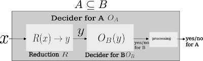
Implicitly this is a two-step process.
- First, instances of $A$ are reduced/transformed into instances of $B$. Therefore $x\in A$ is transformed into $y\in B$. Since $x$ is “reduced/transformed” into $y$, we shall use $R(x)$ to denote instances of $B$.
- Now we perform invocation(s) to the oracle for $B$ to solve for these transformed instances $R(x)$ or $y$.
Depending on the output of the $B$ oracle, we decide our output for the $A$ oracle. We denote this mathematically as $x\in A \iff R(x) \in B$.
The notion of efficiency is twofold.
- Firstly, we look at how efficient the transformation/reduction from $x$ to $R(x)$ is.
- Secondly, for the oracle $O_B$, we are concerned with how many times the oracle is invoked.
The notion of efficiency in transforming $x$ to $R(x)$ has a small caveat, which we explore via an example.
Only the construction of the reduction method $R$ needs to be efficient, and solving $O_B(R(x))$ does not need to be efficient.
For example consider the following C pseudocode:
int A(int x){
	for(;x>12;x++);
	return x; // This is R(x)
}
Writing this piece of code took finite time, and was certainly efficient. However, depending on the value of the input the for loop will never terminate for values of $x>11$. Therefore, this program may become inefficient during runtime. The notion of efficiency we consider during reductions (unlike computational scenarios) is how efficiently we can write the code for function A, and not how efficiently A transforms $x$ into $R(x)$.
Reducing SAT to the Halting Problem
Note: This is a highly technical section, and would need familiarity to the satisfiability problem and the Halting problem. We encourage the reader to familiarize themselves with the formal definitions of these problems first before going through this section. We give an intuitive description of the problems below.
The Halting Problem
Recall the earlier piece of pseudocode with a slight modification.
int A1(int x){
	for(;x>12;x++);
	return x; // This is R(x)
}
int A2(int x){
	for(;x>12;x--);// This loop will always terminate
	return x; // This is R(x)
}
Note A2 will always halt no matter the input, while A1 may never halt depending on the input.
Imagine you would like to design a function $B$ that takes the binary description of any single parameter function $A$ and any arbitrary input $x$, and find out whether $A$ will halt on input $x$.
The Halting problem: Given a Turing Machine $A$ and an arbitrary input $x$, does $A(x)$ halt?
This in effect describes the Halting problem, where $B$ is a universal Turing machine and $A$ can be any Turing Machine. It has been shown that there does not exist any such $B$ which solves this problem. Therefore the Halting problem cannot be decided, and is formally referred to as an undecidable problem.
The SAT Problem
A Boolean formula $f$ accepts as input an $n$-bit string and outputs a $1$ (if it accepts the string), or a $0$ (if it rejects the string). Mathematically, $f:{0,1}^{n}\xrightarrow{}{0,1}$.
The satisfiability(SAT) problem: Given a formula $f$ and an arbitrary $n$ bit string $x\in{0,1}^{n}$, is $f(x)=1$?
Note that the structure of SAT is subsumed by the structure of the Halting problem. If the decider to Halting problem ever halts, we can find out whether $f(x)=1$.
Even though SAT can be quite hard to solve computationally (may have exponential runtime depending on the structure of the formula), we can construct an algorithm to solve it. Therefore, right off the bat, we observe that SAT is easier to solve (it is decidable) than the Halting problem.
The Reduction
Let us finally have a look at how we would reduce SAT to the Halting problem.
Our input $x$ is a
SATformula.We construct a TM (Turing Machine) $T$ which accepts $x$ and does the following:
- $T$ iterates over all possible assignments to find a satisfying assignment.
This may require exponential runtime in the size of the formula. - If $T$ finds a satisfying assignment, it will halt.
- Otherwise, we put $T$ into an infinite loop.
- $T$ iterates over all possible assignments to find a satisfying assignment.
Our reduction $R(x)$ takes the SAT formula $x$ and returns an encoding of the above Turing machine $T$ with $x$. More precisely, we have something like $R(x)=\left<\lfloor T\rfloor,x\right>$. Note that $R(x)$ at this point can be compared to a compiled binary which has not yet been executed.
We pass $R(x)$ to $O_{\text{halt}}$.
- If $O_{\text{halt}}$ returns yes, this implies $T$ halts on input $x$, which in turn implies $x$ has a satisfying assignment. Therefore $R(x)\in\text{HALT}\implies x\in\text{SAT}$.
- If $O_{\text{halt}}$ returns no, then $T$ does not halt on input $x$, which implies that $x$ does not have a satisfying assignment. Therefore $R(x)\notin\text{HALT}\implies x\notin\text{SAT}$. We can take the contrapositive of this expression to obtain $x\in\text{SAT}\implies R(x)\in\text{HALT}$.
In step 2, we are simply constructing the TM $T$, not executing it. The reduction is the transformation of the SAT formula $x$ to an encoding of both the Turing Machine and the SAT formula, which is an instance of the Halting problem (HALT$_{TM}$ requires an arbitrary TM and an input string to the TM).
Taxonomy of Polynomial-time reductions
Here we only consider polynomial-time reductions, i.e.
- the time taken to transform $x$ to $R(x)$, and
- the number of calls to $O_B$ are both polynomial. These are the most commonly studied types of reductions, and we look at three kinds of polynomial-time reductions.
Karp Reductions / poly-time Many-one reductions
These are the most restrictive type of polynomial reductions.
Given a single input $x$, $R(x)$ produces a single instance $y$ such that $x\in A\iff y\in B$. Therefore, we have to perform only one oracle call to $O_B$. The earlier reduction from SAT to HALT was a Karp reduction.
We can choose to strengthen the notion of Karp reductions to include weaker forms of reductions. For example, in logspace many-one reductions, we can compute $R(x)$ using just logarithmic space instead of polynomial time. Even more restrictive notions of reductions consider reductions computable by constant depth circuit classes.
Truth Table Reductions
These are reductions in which given a single input $x$, $R(x)$ produces a constant number of outputs $y_1,y_2,\ldots, y_k$ to $B$. The output $O_A(x)$ can be expressed in terms of a function $f$ that combines the outputs $O_B(y_i)$ for $i\in[1,\ldots,k]$.
Let us assume that $f$ outputs $1$ for the desired combination and $0$ otherwise. $$ x\in A\iff f\left(y_1\in B, y_1\in B,\ldots,y_k\in B\right)=1 $$ Here, $f$ is efficiently computable, and there are a constant ($k$) number of oracle calls to $O_B$.
Let us consider an example. Consider two problems on a graph $G$ with a constant number of vertices $\ell$.
$A$: What is the minimum sized independent set for $G$? $B$: Does $G$ have an independent set of size $k$?
The reduction $A\subseteq B$ would involve looping from $1$ to $\ell$ and querying $B$ each time. The combination function would be an OR function. At the first yes instance of $B$, we return the value as the answer for $A$. If there is no independent set in $G$, the worst number of calls to $O_B$ is $\ell$.
Cook Reductions / poly-time Turing Reductions
Here, we are allowed a polynomial number of oracle calls and polynomial time for transforming the inputs. These are the most general form of reductions, and the other forms of reductions are restrictions of Cook reductions. In the example graph $G$ used for TT reductions, if we assume the number of vertices of $G$ to be a polynomial, then the reduction $A\subseteq B$ using the same exact process would be a Cook reduction.
$A\subseteq_{m} B \implies A\subseteq_{t} B \implies A\subseteq_{T} B$ where, $\subseteq_{m}$ denotes Karp reductions, $\subseteq_{t}$ denotes Truth Table reductions, and $\subseteq_{T}$ denotes Cook reductions.
Aside: From the nature of the examples, we can see that Karp reductions only extend to decision problems (problems with yes/no outputs). In contrast, Cook reductions can accommodate search/relation/optimization problems (problems with a set of outputs).
Basic reductions in Computability Theory
In this section, the reader is assumed to have familiarity with concepts of decidability and undecidability. Let us now proceed with some instances of reductions in computability theory.
Let $A\subseteq B$, and they are decision problems.
- If $A$ is decidable, what can we say about $B$?
- If $A$ is semi-decidable, what can we say about $B$?
- If $A$ is undecidable, what can we say about $B$?
We know that $B$ is at least as hard as $A$ since $A\subseteq B$. Therefore in the first case, $B$ may be decidable, semi-decidable, or undecidable. In the second case, $B$ may be semi-decidable, or undecidable. In the third case, $B$ is undecidable.
The third case is of interest here - To show that a $B$ is undecidable, we must find a reduction from $A$ to $B$, where $A$ is already known to be undecidable. Note (Advanced): The reduction function must itself be a computable function.
Now again, consider $A\subseteq B$ where they are decision problems. We can conclude the following:
- If $B$ is decidable, $A$ is decidable.
- If $B$ is semi-decidable, $A$ is semi-decidable.
- If $A$ is not decidable, then $B$ is not decidable.
- If $A$ is not semi-decidable, then $B$ is not semi-decidable.
- $A\subseteq B$, then $\bar{A}\subseteq \bar{B}$, where $A$ and $B$ are decidable problems.
The first two statements are true, as discussed above, while 3 is the contrapositive of the first statement and the fourth statement is the contrapositive of the second statement. For the fifth statement, the proof is as follows:
$x\in \bar{A} \iff x\notin A \iff R(x)\notin B \iff R(x)\in\bar{B}$. Therefore, $x\in \bar{A} \iff R(x)\in\bar{B}$.
Immediately we see the power of formalizing the notion of reductions.
Notions of reductions in Complexity Theory
This section is for advanced readers only due to the number of prerequisites involved.
A complexity class is a set of computational problems that can be solved using similar amounts of bounded resources (time, space, circuit depth, number of gates, etc.) on a given computational model (Turing machines, cellular automaton, etc.).
The complexity classes P, NP, and PSPACE are closed under Karp and logspace reductions. The complexity classes $L$ and $NL$ are closed only under logspace reductions. Closure has the following semantics - given a problem $A$ in a complexity class C, any problem $B$ such that $B\subseteq A$ is also in C.
We now explore two interesting notions in complexity theory that arise from reductions.
Completeness
For a bounded complexity class,
Complete problems are the hardest problems inside their respective complexity class.
A more formal definition of completeness is as follows:
Given a complexity class $C$ which is closed under reduction $r$, if there exists a problem $A$ in $C$ such that all other problems in $C$ are $r$-reducible to $A$, $A$ is said to be C-complete.
For example, an NP-complete problem is in NP, and all problems in NP are Karp-reducible to it. The notions of PSPACE-completeness and EXPTIME-completeness are similarly defined under Karp-reductions.
The role of reductions in this context can be understood through P-completeness. Consider any non-trivial decision problem in P (trivial problems are akin to constant functions). Every other non-trivial decision problem is Karp-reducible to it. Therefore every non-trivial decision problem is P-complete under Karp-reductions. This definition is essentially the same as P (minus the empty language and $\Sigma^*$). Therefore, we come to the following conclusion:
Under Karp-reductions, the notion of P-completeness is semantically useless.
Therefore, we use weaker forms of reductions such as logspace reductions or reductions using constant depth circuit computable functions to achieve a more meaningful notion of P-completeness.
Self reducibility
Decision problems are yes/no problems where we ask if a solution exists. However, sometimes we also want to solve the corresponding search problem to find a solution (if one exists).
In the context of languages in NP, self-reducibility essentially states that if we can efficiently solve the decision version of a problem, we can also efficiently solve the search/optimization version of the problem. A more formal definition would be as follows - the search version of a problem Cook-reduces (polynomial-time Turing-reduces) to the decision version of the problem. Every NP-complete problem is self-reducible and downward self-reducible.
Conclusion
This write-up aims to demystify a core technique used in theoretical computer science and provide a few contexts for its usage. For a more rigorous and formal introduction to this topic, please check out Michael Sipser’s excellent book “An Introduction to the Theory of Computation.” There are many more things to say about reductions, and this article barely scratches the surface on any of the topics it touches. However, I feel it would be prudent to stop at this point before it becomes any more of a rambling mess than it already is.